Computation of limited commitment model, based on Laczó (2015)

The purpose of this document is to understand how to compute value functions and consumption under risk-sharing with limited commitment. For this, I extensively use the codes by Laczó (2015), which can be downloaded here. Since I am not using her codes directly but rather I used her codes to understand the computational process, our codes look very different and all errors and bugs in the code below are on my own.

1 Model

In this document, I consider a problem of two households, unlike the model in Laczó (2015) that considers many households in a village. As in other studies, Laczó (2015) considers the constrained-efficient consumptioon alocatinos. The social planner solves the following problem:

\[\begin{align*} &\max_{\{c_{it}(s^t)\}} \sum_i \lambda_i \sum_{t = 1}^{\infty} \sum_{s^t} \delta^t \pi(s^t) u_i(c_{it}(s^t)) \\ \text{subject to} &\sum_i c_{it} (s^t) \le \sum_i y_{it}(s_t) \quad \forall s^t, \forall t \\ &\sum_{r = t}^{\infty} \sum_{s^r} \delta^{r - t} \pi(s^r | s^t) u_i(c_{ir}(s^r)) \ge U_{i}^{aut}(s_t) \quad \forall s^t, \forall t, \forall i. \end{align*}\]

Here, the income follows a Markov process and is independent across households. Notice the difference between the history of states up to period \(t\) (\(s^t\)) and the state at period \(t\) (\(s_t\)). The variable \(\lambda_i\) is the Pareto weight of a household \(i\). The last equation is the participation constraints (PCs), whose RHS is the value of autarky and the solution of the following Bellman equation:

\[ U_i^{aut}(s_t) = u_i((1 - \phi) y_{it}(s_t)) + \delta \sum_{s^{t + 1}} \pi(s_{t + 1} | s_t) U_{i}^{aut}(s_{t + 1}), \] where \(\phi\) is the punishment of renege, which is a fraction of consumption each period. It is assumed that savings are absent.

Letting the multiplier on the PC of \(i\) be \(\delta^t \pi(s^t) \mu_i(s^t)\) andd the multiplier on the aggregate resource constraint be \(\delta^t \pi(s^t) \rho(s^t)\), the Lagrangian is

\[ \sum_{t = 1}^{\infty} \sum_{s^t} \delta^t \pi(s^t) \left\{ \sum_i \left[ \lambda_i u_i(c_{it}(s^t)) + \mu_i(s^t) \left( \sum_{r = t}^{\infty} \sum_{s^r} \delta^{r - t} \pi(s^r | s^t) u_i (c_{ir} (s^r)) - U_i^{aut}(s_t) \right) \right] + \rho(s^t) \left( \sum_i \left(y_{it} (s_t) - c_{it} (s^t) \right) \right) \right\} \] With the recursive method in Marcet and Marimon (2019), this Lagrangian can be written as

\[ \sum_{t = 1}^{\infty} \sum_{s^t} \delta^t \pi(s^t) \left\{ \sum_i \left[ M_i (s^{t - 1}) u_i (c_{it} (s^t)) + \mu_i (s^t) (u_i (c_{it} (s^t)) - U_i^{aut} (s_t)) \right] + \rho(s^t) \left( \sum_i \left( y_{it}(s_t) - c_{it} (s^t) \right) \right) \right\}, \]

where \(M_i(s^t) = M_i(s^{t - 1}) + \mu_i(s^t)\) and \(M_i(s^0) = \lambda\). The variable \(M_i(s^t)\) is the current Pareto weight of household \(i\) and is equal to its initial Pareto weight plus the sum of the Lagrange mulipliers on its PCs along the history \(s^t\).

Let \(x_i(s^t) = \frac{M_i(s^t)}{M_v(s^t)}\), the relative Pareto weight of household \(i\) under the history \(s^t\), where the weight of household \(v\) is normalized to \(1\). Then, the vector of relative weights \(x(s^t)\) plays as a role as a co-state variable, and the solution consists of policy functions \(x_{it}(s_t, x_{t - 1})\) and \(c_{it}(s_t, x_{t - 1})\). That is, \(x_{t - 1}\) is a sufficient statistic for the history up to \(t - 1\). The optimality condition is

\[ \frac{u_v'(c_{vt}(s_t, x_{t - 1}))}{u_i'(c_{it}(s_t, x_{t - 1}))} = x_{it}(s_t, x_{t - 1}) \quad \forall i. \]

The value functioon can be written recursively as

\[ V_i(s_t, x_{t - 1}) = u_i (c_{it} (s_t, x_{t - 1})) + \delta \sum_{s_{t + 1}} \pi(s_{t + 1} | s_t) V_i (s_{t + 1}, x_t(s_t, x_{t - 1})). \]

Laczó (2015) argues that, as in Ligon, Thomas, and Worrall (2002), the evolution of relative Pareto weights is fully characterized by state-dependent intervals, which give the weights in the case where PCs are binding.

2 Computation

In this section I conduct a numerical exercise to compute value functions under the limited commitment model with heterogeneous risk preferences.

2.1 Model settings

I simplify the model of Laczó (2015) and consider two households with \(2 \times 2\) states. The income process are iid:

\[ y_1 = [2/3, 4/3],\ y_2 = [2/3, 4/3], \\ \pi_1 = [0.1, 0.9],\ \pi_2 = [0.1, 0.9]. \]

# income shocks and their transition probabilities of the household
inc1 <- c(2/3, 4/3)
P1 <- matrix(rep(c(0.1, 0.9), 2), nrow = 2, byrow = TRUE)

# income shocks and their transition probabilities of the village
inc2 <- c(2/3, 4/3)
P2 <- matrix(rep(c(0.1, 0.9), 2), nrow = 2, byrow = TRUE)

# transition super-matrix of income shocks
R <- kronecker(P2, P1)

# number of states
# (number of income states for a household times
# number of income states for the village)
S <- length(inc1) * length(inc2)

# Income matrix
# (col 1: HH income, col 2: village income)
inc_mat <- as.matrix(expand.grid(inc1, inc2))

# Aggregate income in each state
inc_ag <- rowSums(inc_mat)

I assume the CRRA utility functions:

\[ u_i(c_{it}) = \frac{c_{it}^{1 - \sigma_i} - 1}{1 - \sigma_i}. \]

# Define utility function
util <- function(c, sigma) {
  if (sigma != 1) {
    output = (c ^ (1 - sigma) - 1) / (1 - sigma)
  } else if (sigma == 1) {
    output = log(c)
  }
  return(output)
}
util_prime <- function(c, sigma) c ^ (- sigma)

2.2 Value of autarky

delta <- 0.95 # time discount factor 
sigma1 <- 1.0 # coefficient of relative risk aversion of HH1
sigma2 <- 1.0 # coefficient of relative risk aversion of HH2
pcphi <- 0.0 # punishment under autarky

Uaut_func <- function(
  inc1, P1, inc2, P2,
  delta, sigma1, sigma2, pcphi,
  util, util_prime
  ) {

  # Expected utility under autarky for HH
  U1_aut <- numeric(length = length(inc1))
  i <- 1
  diff <- 1
  while (diff > 1e-12) {
    U1_aut_new <- util((inc1 * (1 - pcphi)), sigma1) + delta * P1 %*% U1_aut
    diff <- max(abs(U1_aut_new - U1_aut))
    U1_aut <- U1_aut_new
    i <- i + 1
  }

  # Expected utility under autarky for village
  U2_aut <- numeric(length = length(inc2))
  i <- 1
  diff <- 1
  while (diff > 1e-12) {
    U2_aut_new <- util((inc2 * (1 - pcphi)), sigma2) + delta * P2 %*% U2_aut
    diff <- max(abs(U2_aut_new - U2_aut))
    U2_aut <- U2_aut_new
    i <- i + 1
  }

  # Since in this case the income process are iid, 
  # values under autarky can be computed in the following way:
  # U1_out = util((1 - pcphi) * inc1, sigma1) + delta / (1 - delta) * P1 %*% util((1 - pcphi) * inc1, sigma1)
  # U2_out = util((1 - pcphi) * inc2, sigma2) + delta / (1 - delta) * P2 %*% util((1 - pcphi) * inc2, sigma2)
  # This way does not work when income processes are autocorrelated, as in the original model of Laczo (2015)

  # Matrix of expected utilities of autarky
  # (col 1: HH, col 2: village)
  Uaut <- expand.grid(U1_aut, U2_aut)

  return(Uaut)
}

Uaut <- Uaut_func(inc1, P1, inc2, P2, delta, sigma1, sigma2, pcphi, util, util_prime)

2.3 Grid of relative Pareto weights and consumption on the grid points

Here, I make the grid of relative Pareto weight of household 1, \(x(s^t)\), on which I compute the values (I use the notation \(x(s^t)\) rather than \(x_i(s^t)\) since there are only two households). The number of grid points is \(200\).

# (Number of grid points on relative Pareto weight) - 1
g <- 199

# The grid points of relative Pareto weights
qmin <- util_prime(max(inc2), sigma2) / util_prime(min(inc1 * (1 - pcphi)), sigma1)
qmax <- util_prime(min(inc2 * (1 - pcphi)), sigma2) / util_prime(max(inc1), sigma1)
q <- exp(seq(log(qmin), log(qmax), length.out = (g + 1)))

Then, I compute consumptions of the household 1 on these grid points. From the optimality condition and the CRRA utility functions, we obtain

\[ \frac{(y_{1t} + y_{2t} - c_{1t})^{- \sigma_2}}{c_{1t}^{- \sigma_1}} = x_{t}. \]

Since there is no closed form solution for this in general, I derive \(c_{1t}\) numerically. However, when \(\sigma_1 = \sigma_2 = \sigma\), the closed-form solution is

\[ c_{1t} = \frac{y_{1t} + y_{2t}}{1 + x_t^{- 1 / \sigma}}. \]

# The grid points of consumption of HH 1
# Consumption is determined by aggregate income (inc_ag) and
# relative Pareto weights (q)
cons1 <- matrix(nrow = S, ncol = (g + 1))
for (k in 1:S) {
  for (l in 1:(g + 1)) {
    if (sigma1 == sigma2) {
      cons1[k, l] <- inc_ag[k] / (1 + q[l]^(- 1 / sigma1))
    } else {
      f = function(w) util_prime((inc_ag[k] - w), sigma2) - q[l] * util_prime(w, sigma1)
      v = uniroot(f, c(1e-5, (inc_ag[k] - 1e-5)), tol = 1e-8, maxiter = 100)
      cons1[k, l] <- v$root
    }
  }
}

2.4 Values under risk-sharing (full)

Now, I compute the values under full risk-sharing, which will be used as the initial values in value function iterations under the limited commitment model. Note that, under full risk sharing, the consumption only depends on the aggregate resources and time-invariate relative Pareto weights. Hence, I numerically solve the following Bellman equation:

\[ V_i^{full}(s_t, x) = u_i(c_{it}(s_t, x)) + \delta \sum_{s^{t + 1}} \pi(s_{t + 1} | s_t) V_{i}^{full}(s_{t + 1}, x). \]

V_full_func <- function(
  inc1, P1, inc2, P2, g,
  R, S, inc_ag, qmin, qmax, q,
  delta, sigma1, sigma2, pcphi,
  util, util_prime, Uaut, cons1
  ) {

  # Value function iterations ================
  # Initial guess is expected utilities under autarky
  V1 <- outer(Uaut[, 1], rep(1, (g + 1)))
  V2 <- outer(Uaut[, 2], rep(1, (g + 1)))
  V1_new <- matrix(nrow = S, ncol = (g + 1))
  V2_new <- matrix(nrow = S, ncol = (g + 1))

  # Obtain value functions by value function iterations
  j <- 1
  diff <- 1
  while (diff > 1e-8 & j < 500) {
    V1_new <- util(cons1, sigma1) + delta * R %*% V1
    V2_new <- util(inc_ag - cons1, sigma2) + delta * R %*% V2
    diff <- max(max(abs(V1_new - V1)), max(abs(V2_new - V2)))
    V1 <- V1_new
    V2 <- V2_new
    j <- j + 1
  }

  V1_full <- V1
  V2_full <- V2

  return(list(V1_full, V2_full))
}

V_full <- V_full_func(
  inc1, P1, inc2, P2, g,
  R, S, inc_ag, qmin, qmax, q,
  delta, sigma1, sigma2, pcphi,
  util, util_prime, Uaut, cons1
)

V1_full <- V_full[[1]]
V2_full <- V_full[[2]]

2.5 Values under risk-sharing (limited commitment)

Next, I derive the state-dependent intervals of relative Pareto weights and calculate values under the model of limited commitment. To derive the intervals, I use the fact that at the limits of the intervals, the PCs are binding. For instance, to compute the lower limit \(\underline{x}^h(s)\), where \(h\) indicates \(h\)’th iteration, the PC of the household 1 is binding:

\[ u_1(c_1^h(s)) + \delta \sum_{s'} \pi(s' | s) V_1^{h - i} (s', \underline{x}^h(s)) = U_1^{aut}(s), \] where the optimality condition is

\[ \frac{u_2'(c_{2}^h(s))}{u_1'(c_{1}^h(s))} = \underline{x}^h(s). \]

Notice that, once the PC binds, the past history, which is summarized by \(x_{t - 1}\), does not matter. This property is called “amnesia” (Kocherlakota (1996)). Since \(\underline{x}^h(s)\) may not be on the grid \(q\), linear interpolation is used to compute \(V_1^{h - 1}(s', \underline{x}^h(s))\).

Similarly, \(\overline{x}^h(s)\) is computed using the binding PC of the household 2

\[ u_2(c_2^h(s)) + \delta \sum_{s'} \pi(s' | s) V_2^{h - i} (s', \overline{x}^h(s)) = U_2^{aut}(s), \] where the optimality condition is

\[ \frac{u_2'(c_{2}^h(s))}{u_1'(c_{1}^h(s))} = \overline{x}^h(s). \]

After deriving these limits of intervals,

1. for relative Pareto weights below \(\underline{x}^h(s)\), compute consumption of HH1 based on \(\underline{x}^h(s)\) and let its value be \(U_1^{aut}\);
2. for relative Pareto weights above \(\overline{x}^h(s)\), compute consumption of HH1 based on \(\overline{x}^h(s)\) and let the value of HH2 be \(U_2^{aut}\);
3. for other relative Pareto weights, use them to compute consumption of HH1 and the values of households.

By iterating these steps, we can calculate the value functions of households and limits of intervals.

V_lc_func <- function(
  inc1, P1, inc2, P2, g,
  R, S, inc_ag, qmin, qmax, q,
  delta, sigma1, sigma2, pcphi,
  util, util_prime, Uaut, cons1, 
  V1_full, V2_full
  ) {

  # Value function iterations ================
  # Initial guess is expected utilities under full risk sharing
  V1 <- V1_full
  V2 <- V2_full
  V1_new <- matrix(nrow = S, ncol = (g + 1))
  V2_new <- matrix(nrow = S, ncol = (g + 1))

  diff <- 1
  iter <- 1
  maxiter <- 1000
  while ((diff > 1e-12) && (iter <= maxiter)) {

    cons1_lc <- cons1 # consumption of HH 1 under LC
    x_lc <- outer(rep(1, S), q)
    x_int <- matrix(nrow = S, ncol = 2) # matrix of bounds of intervals
  
    # First, ignore enforceability and just update the value functions
    # using the values at the previous iteration
    V1_new <- util(cons1, sigma1) + delta * R %*% V1
    V2_new <- util(inc_ag - cons1, sigma2) + delta * R %*% V2
    
    # Now check enforceability at each state
    for (k in 1:S) {
      
      # This function calculate the difference between the value when the relative Pareto weight is x
      # and the value of autarky. This comes from the equation (1) in the supplementary material of
      # Laczo (2015). Used to calculate the lower bound of the interval.
      calc_diff_val_aut_1 <- function(x) {
        # Calculate consumption of HH 1 at a relative Pareto weight x
        if (sigma1 == sigma2) {
          cons_x <- inc_ag[k] / (1 + x^(- 1 / sigma1))
        } else {
          f <- function(w) util_prime(inc_ag[k] - w, sigma2) / util_prime(w, sigma1) - x
          cons_x <- uniroot(f, c(1e-6, (inc_ag[k] - 1e-6)), tol = 1e-10, maxiter = 300)$root
        }
        
        # Index of the point on the grid of relative Pareto weights (q) closest to x
        q_ind <- which.min(abs(x - q))
        if (x > q[q_ind]) {
          q_ind <- q_ind + 1
        }
        
        # Value functions of HH 1 under the relative Pareto weights x
        # (I use interpolation since x might not be on the grid q)
        V1_x <- apply(V1, 1, function(y) approxfun(q, y, rule = 2)(x))
        
        # difference between 
        diff <- util(cons_x, sigma1) + delta * R[k,] %*% V1_x - Uaut[k, 1]
        return(diff)
      }
      
      # Similarly, this function is used to calculate the upper bound.
      calc_diff_val_aut_2 <- function(x) {
        # Calculate consumption of HH 1 at a relative Pareto weight x
        if (sigma1 == sigma2) {
          cons_x <- inc_ag[k] / (1 + x^(- 1 / sigma1))
        } else {
          f <- function(w) util_prime(inc_ag[k] - w, sigma2) / util_prime(w, sigma1) - x
          cons_x <- uniroot(f, c(1e-6, (inc_ag[k] - 1e-6)), tol = 1e-10, maxiter = 300)$root
        }
        
        # Index of the point on the grid of relative Pareto weights (q) closest to x
        q_ind <- which.min(abs(x - q))
        if (x > q[q_ind]) {
          q_ind <- q_ind + 1
        }
        
        # Value functions of HH 1 under the relative Pareto weights x
        # (I use interpolation since x might not be on the grid q)
        V2_x <- apply(V2, 1, function(y) approxfun(q, y, rule = 2)(x))
        
        # difference between 
        diff <- util(inc_ag[k] - cons_x, sigma2) + delta * R[k,] %*% V2_x - Uaut[k, 2]
        return(diff)
      }   
      
      # If the relative Pareto weight is too low and violates the PC, then
      # set the relative Pareto weight to the lower bound of the interval, and
      # HH1 gets the value under autarky.
      if ((calc_diff_val_aut_1(qmax) > 0) && calc_diff_val_aut_1(qmin) < 0) {
        
        # Derive the relative Pareto weight that satisfies the equation (1)
        # in the supplementary material of Laczo (2015)
        x_low <- uniroot(calc_diff_val_aut_1, c(qmin, qmax), tol = 1e-10, maxiter = 300)$root
        x_int[k, 1] <- x_low
        
        # Index of the point on the grid of relative Pareto weights (q) closest to x_low
        q_ind_low <- which.min(abs(x_low - q))
        if (x_low > q[q_ind_low]) {
          q_ind_low <- q_ind_low + 1
        }
        x_lc[k, 1:q_ind_low] <- x_low
        
        # Value functions of HH 2 under the relative Pareto weights x
        # (I use interpolation since x_low might not be on the grid q)
        V2_x <- apply(V2, 1, function(y) approxfun(q, y, rule = 2)(x_low))
        
        # Calculate consumption of HH 1 at a relative Pareto weight x_low
        if (sigma1 == sigma2) {
          cons_x_low <- inc_ag[k] / (1 + x_low^(- 1 / sigma1))
        } else {
          f <- function(w) util_prime(inc_ag[k] - w, sigma2) / util_prime(w, sigma1) - x_low
          cons_x_low <- uniroot(f, c(1e-6, (inc_ag[k] - 1e-6)), tol = 1e-10, maxiter = 300)$root
        }
        
        cons1_lc[k, 1:q_ind_low] <- cons_x_low
        V1_new[k, 1:q_ind_low] <- Uaut[k, 1]
        V2_new[k, 1:q_ind_low] <- util((inc_ag[k] - cons_x_low), sigma2) + delta * R[k,] %*% V2_x
      } else if (calc_diff_val_aut_1(qmax) <= 0) {
        V1_new[k,] <- Uaut[k, 1]
        V2_new[k,] <- Uaut[k, 2]
        x_int[k, 1] <- qmax
        x_lc[k,] <- qmax
        q_ind_low <- g + 2
      } else if (calc_diff_val_aut_1(qmin) >= 0) {
        x_int[k, 1] <- qmin
        q_ind_low <- 0
      }
    
      # If the relative Pareto weight is too high and violates the PC, then
      # set the relative Pareto weight to the upper bound of the interval, and
      # HH2 gets the value under autarky.
      if (q_ind_low <= (g + 1)) {
        if ((calc_diff_val_aut_2(qmin) > 0) && calc_diff_val_aut_2(qmax) < 0) {
          
          # Derive the relative Pareto weight that satisfies the equation (2)
          # in the supplementary material of Laczo (2015)
          x_high <- uniroot(calc_diff_val_aut_2, c(qmin, qmax), tol = 1e-10, maxiter = 300)$root
          x_int[k, 2] <- x_high
          
          # Index of the point on the grid of relative Pareto weights (q) closest to x_low
          q_ind_high <- which.min(abs(x_high - q))
          if (x_high > q[q_ind_high]) {
            q_ind_high <- q_ind_high + 1
          }
          x_lc[k, 1:q_ind_high] <- x_high
          
          # Value functions of HH 2 under the relative Pareto weights x
          # (I use interpolation since x_high might not be on the grid q)
          V1_x <- apply(V1, 1, function(y) approxfun(q, y, rule = 2)(x_high))
          
          # Calculate consumption of HH 1 at a relative Pareto weight x_high
          if (sigma1 == sigma2) {
            cons_x_high <- inc_ag[k] / (1 + x_high^(- 1 / sigma1))
          } else {
            f <- function(w) util_prime(inc_ag[k] - w, sigma2) / util_prime(w, sigma1) - x_high
            cons_x_high <- uniroot(f, c(1e-6, (inc_ag[k] - 1e-6)), tol = 1e-10, maxiter = 300)$root
          }
          
          cons1_lc[k, q_ind_high:(g + 1)] <- cons_x_high
          V1_new[k, q_ind_high:(g + 1)] <- util(cons_x_high, sigma1) + delta * R[k,] %*% V1_x
          V2_new[k, q_ind_high:(g + 1)] <- Uaut[k, 2]
        } else if (calc_diff_val_aut_2(qmin) <= 0) {
          V1_new[k,] <- Uaut[k, 1]
          V2_new[k,] <- Uaut[k, 2]
          x_int[k, 2] <- qmin
          x_lc[k,] <- qmin
          q_ind_high <- 0
        } else if (calc_diff_val_aut_2(qmax) >= 0) {
          x_int[k, 2] <- qmax
          q_ind_high <- g + 2
        }
      }
      
      # The case where the relative Pareto weight does not violate PC
      if ((q_ind_low + 1) < (q_ind_high - 1)) {
        V1_new[k, (q_ind_low + 1):(q_ind_high - 1)] <- 
          util(cons1[k, (q_ind_low + 1):(q_ind_high - 1)], sigma1) + 
          delta * R[k,] %*% V1[, (q_ind_low + 1):(q_ind_high - 1)]
        V2_new[k, (q_ind_low + 1):(q_ind_high - 1)] <- 
          util(inc_ag[k] - cons1[k, (q_ind_low + 1):(q_ind_high - 1)], sigma2) + 
          delta * R[k,] %*% V2[, (q_ind_low + 1):(q_ind_high - 1)]
      }
      
    }
    
    diff <- max(max(abs(V1_new - V1)), max(abs(V2_new - V2)))
    V1 <- V1_new
    V2 <- V2_new
    iter <- iter + 1
    
  }

  if (iter == maxiter) {
    print("Reached the maximum limit of iterations!")
  }

  return(list(V1, V2, x_int))
}

2.6 Make a pipeline based on the functions defined above

V_lc_all_func <- function(
  inc1, P1, inc2, P2, g,
  delta, sigma1, sigma2, pcphi,
  util, util_prime
  ) {

  # Pre settings ====================
  # transition super-matrix of income shocks
  R <- kronecker(P2, P1)

  # number of states
  # (number of income states for a household times
  # number of income states for the village)
  S <- length(inc1) * length(inc2)

  # Aggregate income in each state
  inc_ag <- rowSums(expand.grid(inc1, inc2))

  # The grid points of relative Pareto weights
  qmin <- util_prime(max(inc2), sigma2) / util_prime(min(inc1 * (1 - pcphi)), sigma1)
  qmax <- util_prime(min(inc2 * (1 - pcphi)), sigma2) / util_prime(max(inc1), sigma1)
  q <- exp(seq(log(qmin), log(qmax), length.out = (g + 1)))

  # The grid points of consumption of HH 1
  # Consumption is determined by aggregate income (inc_ag) and
  # relative Pareto weights (q)
  cons1 <- matrix(nrow = S, ncol = (g + 1))
  for (k in 1:S) {
    for (l in 1:(g + 1)) {
      if (sigma1 == sigma2) {
        cons1[k, l] <- inc_ag[k] / (1 + q[l]^(- 1 / sigma1))
      } else {
        f = function(w) util_prime((inc_ag[k] - w), sigma2) - q[l] * util_prime(w, sigma1)
        v = uniroot(f, c(1e-5, (inc_ag[k] - 1e-5)), tol = 1e-8, maxiter = 100)
        cons1[k, l] <- v$root
      }
    }
  }

  # Matrix of expected utilities of autarky
  # (col 1: HH, col 2: village)
  Uaut <- Uaut_func(inc1, P1, inc2, P2, delta, sigma1, sigma2, pcphi, util, util_prime)

  # Values under full risk-sharing
  V_full <- V_full_func(
    inc1, P1, inc2, P2, g,
    R, S, inc_ag, qmin, qmax, q,
    delta, sigma1, sigma2, pcphi,
    util, util_prime, Uaut, cons1
  )

  V1_full <- V_full[[1]]
  V2_full <- V_full[[2]]

  # Values under risk-sharing with dynamic limited commitment
  V_lc <- V_lc_func(
    inc1, P1, inc2, P2, g,
    R, S, inc_ag, qmin, qmax, q,
    delta, sigma1, sigma2, pcphi,
    util, util_prime, Uaut, cons1,
    V1_full, V2_full
    )

  V1_lc <- V_lc[[1]]
  V2_lc <- V_lc[[2]]
  x_int_lc <- V_lc[[3]]

  return(list(V1_full, V2_full, V1_lc, V2_lc, x_int_lc))
}

2.7 Sanity test: replication of Figure 1 in Ligon, Thomas, and Worrall (2002)

For the sanity test of this function, I use it to replicate the Figure 1 in Ligon, Thomas, and Worrall (2002). Here I use the parameter values in the original paper. I choose the income process \((y_l, y_h) = (2/3, 4/3)\) and \((p_l, p_h) = (0.1, 0.9)\) for both households so that the mean is \(1\) and the ratio \(y_l / y_h\) is 1/2 as in the paper. Also, the penalty under autarky is absent as in the original numerical exercise.

# income shocks and their transition probabilities of the household
inc1 <- c(2/3, 4/3)
P1 <- matrix(rep(c(0.1, 0.9), 2), nrow = 2, byrow = TRUE)

# income shocks and their transition probabilities of the village
inc2 <- c(2/3, 4/3)
P2 <- matrix(rep(c(0.1, 0.9), 2), nrow = 2, byrow = TRUE)

sigma1 <- 1.0 # coefficient of relative risk aversion of HH1
sigma2 <- 1.0 # coefficient of relative risk aversion of HH2
pcphi <- 0.0 # punishment under autarky

# (Number of grid points on relative Pareto weight) - 1
g <- 399

# Define utility function
util <- function(c, sigma) {
  if (sigma != 1) {
    output = (c ^ (1 - sigma) - 1) / (1 - sigma)
  } else {
    output = log(c)
  }
  return(output)
}
util_prime <- function(c, sigma) c ^ (- sigma)
  
# Calculate values and intervals at different delta values
delta_seq <- seq(0.8, 0.999, by = 0.002)

output <- vector(mode = "list", length = length(delta_seq))
for (i in seq_along(delta_seq)) {
  output[[i]] <- V_lc_all_func(
     inc1, P1, inc2, P2, g, 
     delta_seq[i], sigma1, sigma2, pcphi, util, util_prime
  )
}

saveRDS(output, file.path("RDSfiles/laczo2015_dynamic_lc_output.rds"))

x_int_array = array(NA, dim = c(S, 2, length(delta_seq)))
for (i in seq_along(delta_seq)) {
  x_int_array[,,i] <- output[[i]][[5]]
}

ggplot() +
  geom_line(aes(delta_seq, log(x_int_array[1,1,]), color = "a")) + 
  geom_line(aes(delta_seq, log(x_int_array[1,2,]), color = "b")) + 
  geom_line(aes(delta_seq, log(x_int_array[2,1,]), color = "c")) + 
  geom_line(aes(delta_seq, log(x_int_array[2,2,]), color = "d")) +
  geom_line(aes(delta_seq, log(x_int_array[3,1,]), color = "e")) +
  geom_line(aes(delta_seq, log(x_int_array[3,2,]), color = "f")) +
  geom_line(aes(delta_seq, log(x_int_array[4,1,]), color = "g")) +
  geom_line(aes(delta_seq, log(x_int_array[4,2,]), color = "h")) +
  coord_cartesian(xlim = c(0.8, 1.0), ylim = c(log(inc1[1] / inc1[2]), log(inc1[2] / inc1[1]))) +
  geom_ribbon(aes(x = delta_seq,
                  ymin = log(x_int_array[1,1,]),
                  ymax = log(x_int_array[1,2,])),
                  fill = "blue", alpha = 0.2) +
  geom_ribbon(aes(x = delta_seq,
                  ymin = log(x_int_array[2,1,]),
                  ymax = log(x_int_array[2,2,])),
                  fill = "red", alpha = 0.2) +
  geom_ribbon(aes(x = delta_seq,
                  ymin = log(x_int_array[3,1,]),
                  ymax = log(x_int_array[3,2,])),
                  fill = "green", alpha = 0.2) +
  geom_ribbon(aes(x = delta_seq,
                  ymin = log(x_int_array[4,1,]),
                  ymax = log(x_int_array[4,2,])),
                  fill = "yellow", alpha = 0.2) +
  scale_color_manual(
    name = "End-points", 
    values = c(
      "blue",
      "purple",
      "brown",
      "red",
      "yellow",
      "green",
      "orange",
      "gray"
      ), 
    labels = unname(TeX(c(
      "$\\underline{x}_{ll}$",
      "$\\bar{x}_{ll}$",
      "$\\underline{x}_{hl}$",
      "$\\bar{x}_{hl}$",
      "$\\underline{x}_{lh}$",
      "$\\bar{x}_{lh}$",
      "$\\underline{x}_{hh}$",
      "$\\bar{x}_{hh}$"
      )))
    ) +
  xlab("Discount factor (delta)") +
  ylab("log of the relative Pareto weights (x)")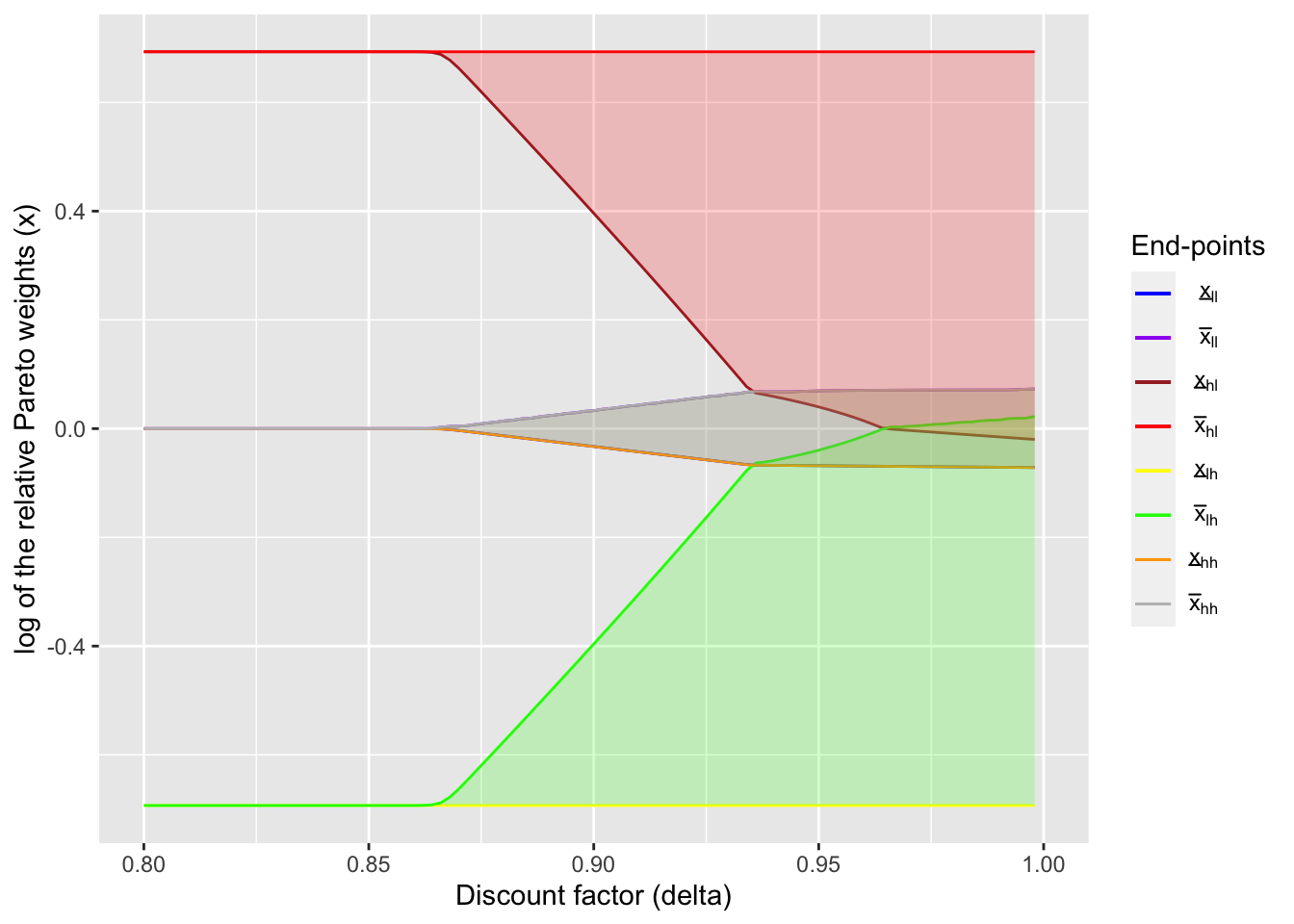

2.8 Bonus: Static limited commitment

Now that I could replicate the figure in Ligon, Thomas, and Worrall (2002), here I will create a similar graph, but under static limited commitment (Coate and Ravallion (1993)). Unlike in dynamic limited commitment model, the initial relative Paretow weight, \(x_0\), plays an important role to determine the transfers. Since past history does not matter in the static limited commitment model, the value function can be written as

\[ V_i(s) = u_i(c_i(s, x_s)) + \delta \sum_{s'} \pi(s'|s) V_i(s'), \] where \(c_i(s, x)\) is a policy function and \(x_s\) is the relative Pareto weight determined by the following rule (Ligon, Thomas, and Worrall (2002)):

\[ x_s = \begin{cases} \overline{x}_s & \text{if } \overline{x}_s < x_0 \\ x_0 & \text{if } \underline{x}_s \le x_0 \le \overline{x}_s \\ \underline{x}_s & \text{if } x_0 < \underline{x}_s. \end{cases} \]

Hence, the limits of state-dependent intervals and the initial relative Pareto weights fully characterize the transfer schedule. The end-points can be derived in the similar way before. For example, I derive \(\underline{x}_s\) using

\[ u_1(c_1(s)) + \delta \sum_{s'} \pi(s'|s) V_1(s') = U_1^{aut}(s) \]

and the optimality condition

\[ \frac{u_2'(c_{2}(s))}{u_1'(c_{1}(s))} = \underline{x}(s). \]

Similarly, I derive \(\underline{x}_s\) using

\[ u_2(c_2(s)) + \delta \sum_{s'} \pi(s'|s) V_2(s') = U_2^{aut}(s) \]

and the optimality condition

\[ \frac{u_2'(c_{2}(s))}{u_1'(c_{1}(s))} = \overline{x}(s). \]

After deriving these limits of intervals,

1. if \(x_0 < \underline{x}(s)\), compute consumption of HH1 based on \(\underline{x}(s)\), let its value be \(U_1^{aut}\), and calculate the value of HH2 using the derived consumption and aggregate income;
2. if \(x_0 > \overline{x}(s)\), compute consumption of HH1 based on \(\overline{x}(s)\), let the value of HH2 be \(U_2^{aut}\), and calculate the value of HH1 using the derived consumption and aggregate income;
3. otherwise, use \(x_0\) to compute consumption of HH1 and the values of households.

By iterating these steps, we can calculate the value functions of households and limits of intervals.

V_static_lc_func <- function(
  inc1, P1, inc2, P2, g,
  R, S, inc_ag, qmin, qmax, q,
  delta, sigma1, sigma2, pcphi,
  util, util_prime, Uaut, cons1, 
  V1_full, V2_full, x0
  ) {

  
  # The grid point closest to the initial relative Pareto weight
  x0_close <- which.min(abs(x0 - q))
  # Value function iterations ================
  # Initial guess is expected utilities under full risk sharing
  V1 <- V1_full[, x0_close]
  V2 <- V2_full[, x0_close]
  V1_new <- vector(mode = "numeric", length = S)
  V2_new <- vector(mode = "numeric", length = S)

  diff <- 1
  iter <- 1
  maxiter <- 1000
  while ((diff > 1e-12) && (iter <= maxiter)) {

    cons1_lc <- cons1 # consumption of HH 1 under LC
    cons1_x0 <- cons1[, x0_close]
    # x_lc <- outer(rep(1, S), q)
    x_int <- matrix(nrow = S, ncol = 2) # matrix of bounds of intervals
  
    # Now check enforceability at each state
    for (k in 1:S) {
      
      # This function calculate the difference between the value when the relative Pareto weight is x
      # and the value of autarky. This comes from the equation (1) in the supplementary material of
      # Laczo (2015). Used to calculate the lower bound of the interval.
      calc_diff_val_aut_1 <- function(x) {
        # Calculate consumption of HH 1 at a relative Pareto weight x
        if (sigma1 == sigma2) {
          cons_x <- inc_ag[k] / (1 + x^(- 1 / sigma1))
        } else {
          f <- function(w) util_prime(inc_ag[k] - w, sigma2) / util_prime(w, sigma1) - x
          cons_x <- uniroot(f, c(1e-6, (inc_ag[k] - 1e-6)), tol = 1e-10, maxiter = 300)$root
        }
        
        # difference between 
        diff <- util(cons_x, sigma1) + delta * R[k,] %*% V1 - Uaut[k, 1]
        return(diff)
      }
      
      # Similarly, this function is used to calculate the upper bound.
      calc_diff_val_aut_2 <- function(x) {
        # Calculate consumption of HH 1 at a relative Pareto weight x
        if (sigma1 == sigma2) {
          cons_x <- inc_ag[k] / (1 + x^(- 1 / sigma1))
        } else {
          f <- function(w) util_prime(inc_ag[k] - w, sigma2) / util_prime(w, sigma1) - x
          cons_x <- uniroot(f, c(1e-6, (inc_ag[k] - 1e-6)), tol = 1e-10, maxiter = 300)$root
        }
        
        # difference between 
        diff <- util(inc_ag[k] - cons_x, sigma2) + delta * R[k,] %*% V2 - Uaut[k, 2]
        return(diff)
      }   
      
      # If the relative Pareto weight is too low and violates the PC, then
      # set the relative Pareto weight to the lower bound of the interval, and
      # HH1 gets the value under autarky.
        
      # Derive the relative Pareto weight that satisfies the equation (1)
      # in the supplementary material of Laczo (2015)
      if ((calc_diff_val_aut_1(qmax) >= 0) && (calc_diff_val_aut_1(qmin) <= 0)) {
        x_low <- uniroot(calc_diff_val_aut_1, c(qmin, qmax), tol = 1e-10, maxiter = 300)$root
        x_int[k, 1] <- x_low
      } else if (calc_diff_val_aut_1(qmax) < 0){
        x_low <- qmax
        x_int[k, 1] <- qmax
      } else if (calc_diff_val_aut_1(qmin) > 0){
        x_low <- qmin
        x_int[k, 1] <- qmin
      }
      
      # Calculate consumption of HH 1 at a relative Pareto weight x_low
      if (sigma1 == sigma2) {
        cons_x_low <- inc_ag[k] / (1 + x_low^(- 1 / sigma1))
      } else {
        f <- function(w) util_prime(inc_ag[k] - w, sigma2) / util_prime(w, sigma1) - x_low
        cons_x_low <- uniroot(f, c(1e-6, (inc_ag[k] - 1e-6)), tol = 1e-10, maxiter = 300)$root
      }
      
      # Derive the relative Pareto weight that satisfies the equation (2)
      # in the supplementary material of Laczo (2015)
      if ((calc_diff_val_aut_2(qmin) >= 0) && calc_diff_val_aut_2(qmax) <= 0) {
        x_high <- uniroot(calc_diff_val_aut_2, c(qmin, qmax), tol = 1e-10, maxiter = 300)$root
        x_int[k, 2] <- x_high
      } else if (calc_diff_val_aut_2(qmin) < 0){
        x_high <- qmin
        x_int[k, 2] <- qmin
      } else if (calc_diff_val_aut_2(qmax) > 0){
        x_high <- qmax
        x_int[k, 2] <- qmax
      }
      
      # Calculate consumption of HH 1 at a relative Pareto weight x_low
      if (sigma1 == sigma2) {
        cons_x_high <- inc_ag[k] / (1 + x_high^(- 1 / sigma1))
      } else {
        f <- function(w) util_prime(inc_ag[k] - w, sigma2) / util_prime(w, sigma1) - x_high
        cons_x_high <- uniroot(f, c(1e-6, (inc_ag[k] - 1e-6)), tol = 1e-10, maxiter = 300)$root
      }
      
      if (q[x0_close] < x_low) {
        V1_new[k] <- Uaut[k, 1]
        V2_new[k] <- util((inc_ag[k] - cons_x_low), sigma2) + delta * R[k,] %*% V2
      } else if (q[x0_close] > x_high) {
        V1_new[k] <- util(cons_x_high, sigma1) + delta * R[k,] %*% V1
        V2_new[k] <- Uaut[k, 2]
      } else {
        V1_new[k] <- util(cons1_x0[k], sigma1) + delta * R[k,] %*% V1
        V2_new[k] <- util((inc_ag[k] - cons1_x0[k]), sigma2) + delta * R[k,] %*% V2
      }
      
      
    }
    
    diff <- max(max(abs(V1_new - V1)), max(abs(V2_new - V2)))
    V1 <- V1_new
    V2 <- V2_new
    iter <- iter + 1
    
  }

  if (iter == maxiter) {
    print("Reached the maximum limit of iterations!")
  }

  return(list(V1, V2, x_int))
}

2.8.1 Make a pipeline based on the functions defined above

V_static_lc_all_func <- function(
  inc1, P1, inc2, P2, g,
  delta, sigma1, sigma2, pcphi,
  util, util_prime, x0
  ) {

  # Pre settings ====================
  # transition super-matrix of income shocks
  R <- kronecker(P2, P1)

  # number of states
  # (number of income states for a household times
  # number of income states for the village)
  S <- length(inc1) * length(inc2)

  # Aggregate income in each state
  inc_ag <- rowSums(expand.grid(inc1, inc2))

  # The grid points of relative Pareto weights
  qmin <- util_prime(max(inc2), sigma2) / util_prime(min(inc1 * (1 - pcphi)), sigma1)
  qmax <- util_prime(min(inc2 * (1 - pcphi)), sigma2) / util_prime(max(inc1), sigma1)
  q <- exp(seq(log(qmin), log(qmax), length.out = (g + 1)))

  # The grid points of consumption of HH 1
  # Consumption is determined by aggregate income (inc_ag) and
  # relative Pareto weights (q)
  cons1 <- matrix(nrow = S, ncol = (g + 1))
  for (k in 1:S) {
    for (l in 1:(g + 1)) {
      if (sigma1 == sigma2) {
        cons1[k, l] <- inc_ag[k] / (1 + q[l]^(- 1 / sigma1))
      } else {
        f = function(w) util_prime((inc_ag[k] - w), sigma2) - q[l] * util_prime(w, sigma1)
        v = uniroot(f, c(1e-5, (inc_ag[k] - 1e-5)), tol = 1e-12, maxiter = 300)
        cons1[k, l] <- v$root
      }
    }
  }

  # Matrix of expected utilities of autarky
  # (col 1: HH, col 2: village)
  Uaut <- Uaut_func(inc1, P1, inc2, P2, delta, sigma1, sigma2, pcphi, util, util_prime)

  # Values under full risk-sharing
  V_full <- V_full_func(
    inc1, P1, inc2, P2, g,
    R, S, inc_ag, qmin, qmax, q,
    delta, sigma1, sigma2, pcphi,
    util, util_prime, Uaut, cons1
  )

  V1_full <- V_full[[1]]
  V2_full <- V_full[[2]]

  # Values under risk-sharing with dynamic limited commitment
  V_lc <- V_static_lc_func(
    inc1, P1, inc2, P2, g,
    R, S, inc_ag, qmin, qmax, q,
    delta, sigma1, sigma2, pcphi,
    util, util_prime, Uaut, cons1, 
    V1_full, V2_full, x0
    )

  V1_lc <- V_lc[[1]]
  V2_lc <- V_lc[[2]]
  x_int_lc <- V_lc[[3]]
  log(x_int_lc)

  return(list(V1_full, V2_full, V1_lc, V2_lc, x_int_lc))
}

2.8.2 Create a figure

# income shocks and their transition probabilities of the household
inc1 <- c(2/3, 4/3)
P1 <- matrix(rep(c(0.1, 0.9), 2), nrow = 2, byrow = TRUE)

# income shocks and their transition probabilities of the village
inc2 <- c(2/3, 4/3)
P2 <- matrix(rep(c(0.1, 0.9), 2), nrow = 2, byrow = TRUE)

sigma1 <- 1.0 # coefficient of relative risk aversion of HH1
sigma2 <- 1.0 # coefficient of relative risk aversion of HH2
pcphi <- 0.0 # punishment under autarky

# (Number of grid points on relative Pareto weight) - 1
g <- 1990

# Define utility function
util <- function(c, sigma) {
  if (sigma != 1) {
    output = (c ^ (1 - sigma) - 1) / (1 - sigma)
  } else {
    output = log(c)
  }
  return(output)
}
util_prime <- function(c, sigma) c ^ (- sigma)

x0 <- 1
  
# Calculate values and intervals at different delta values
delta_seq <- seq(0.8, 0.999, by = 0.002)

static_output <- vector(mode = "list", length = length(delta_seq))
for (i in seq_along(delta_seq)) {
  static_output[[i]] <- V_static_lc_all_func(
     inc1, P1, inc2, P2, g, 
     delta_seq[i], sigma1, sigma2, pcphi, 
     util, util_prime, x0
  )
}

saveRDS(static_output, file.path("RDSfiles/laczo2015_static_lc_output.rds"))

x_int_array = array(NA, dim = c(S, 2, length(delta_seq)))
for (i in seq_along(delta_seq)) {
  x_int_array[,,i] <- static_output[[i]][[5]]
}

ggplot() +
  geom_line(aes(delta_seq, log(x_int_array[1,1,]), color = "a")) + 
  geom_line(aes(delta_seq, log(x_int_array[1,2,]), color = "b")) + 
  geom_line(aes(delta_seq, log(x_int_array[2,1,]), color = "c")) + 
  geom_line(aes(delta_seq, log(x_int_array[2,2,]), color = "d")) +
  geom_line(aes(delta_seq, log(x_int_array[3,1,]), color = "e")) +
  geom_line(aes(delta_seq, log(x_int_array[3,2,]), color = "f")) +
  geom_line(aes(delta_seq, log(x_int_array[4,1,]), color = "g")) +
  geom_line(aes(delta_seq, log(x_int_array[4,2,]), color = "h")) +
  coord_cartesian(xlim = c(0.8, 1.0), ylim = c(log(inc1[1] / inc1[2]), log(inc1[2] / inc1[1]))) +
  geom_ribbon(aes(x = delta_seq,
                  ymin = log(x_int_array[1,1,]),
                  ymax = log(x_int_array[1,2,])),
                  fill = "blue", alpha = 0.2) +
  geom_ribbon(aes(x = delta_seq,
                  ymin = log(x_int_array[2,1,]),
                  ymax = log(x_int_array[2,2,])),
                  fill = "red", alpha = 0.2) +
  geom_ribbon(aes(x = delta_seq,
                  ymin = log(x_int_array[3,1,]),
                  ymax = log(x_int_array[3,2,])),
                  fill = "green", alpha = 0.2) +
  geom_ribbon(aes(x = delta_seq,
                  ymin = log(x_int_array[4,1,]),
                  ymax = log(x_int_array[4,2,])),
                  fill = "orange", alpha = 0.2) +
  scale_color_manual(
    name = "End-points", 
    values = c(
      "blue",
      "purple",
      "brown",
      "red",
      "yellow",
      "green",
      "orange",
      "gray"
      ), 
    labels = unname(TeX(c(
      "$\\underline{x}_{ll}$",
      "$\\bar{x}_{ll}$",
      "$\\underline{x}_{hl}$",
      "$\\bar{x}_{hl}$",
      "$\\underline{x}_{lh}$",
      "$\\bar{x}_{lh}$",
      "$\\underline{x}_{hh}$",
      "$\\bar{x}_{hh}$"
      )))
    ) +
  xlab("Discount factor (delta)") +
  ylab("log of the relative Pareto weights (x)")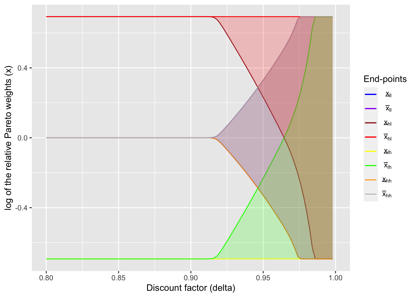

2.9 Bonus 2: Comparative statics in Laczó (2014)

Here, for fun, I replicate Figure 1 in Laczó (2014), which sees how such intervals change with the degree of risk aversion.

# income shocks and their transition probabilities of the household
inc1 <- c(2/3, 4/3)
P1 <- matrix(rep(c(0.1, 0.9), 2), nrow = 2, byrow = TRUE)

# income shocks and their transition probabilities of the village
inc2 <- c(2/3, 4/3)
P2 <- matrix(rep(c(0.1, 0.9), 2), nrow = 2, byrow = TRUE)

sigma1 <- 1.5 # coefficient of relative risk aversion of HH1
sigma2 <- 1.5 # coefficient of relative risk aversion of HH2
pcphi <- 0.0 # punishment under autarky

# (Number of grid points on relative Pareto weight) - 1
g <- 599

# Define utility function
util <- function(c, sigma) {
  if (sigma != 1) {
    output = (c ^ (1 - sigma) - 1) / (1 - sigma)
  } else {
    output = log(c)
  }
  return(output)
}
util_prime <- function(c, sigma) c ^ (- sigma)
  
# Calculate values and intervals at different delta values
delta_seq <- seq(0.8, 0.999, by = 0.002)

laczo2014_output <- vector(mode = "list", length = length(delta_seq))
for (i in seq_along(delta_seq)) {
  laczo2014_output[[i]] <- V_lc_all_func(
     inc1, P1, inc2, P2, g, 
     delta_seq[i], sigma1, sigma2, pcphi, util, util_prime
  )
}

saveRDS(laczo2014_output, file.path("RDSfiles/laczo2014_dynamic_lc_output.rds"))

x_int_array_1 = array(NA, dim = c(S, 2, length(delta_seq)))
for (i in seq_along(delta_seq)) {
  x_int_array_1[,,i] <- output[[i]][[5]]
}

x_int_array_15 = array(NA, dim = c(S, 2, length(delta_seq)))
for (i in seq_along(delta_seq)) {
  x_int_array_15[,,i] <- laczo2014_output[[i]][[5]]
}

ggplot() +
  geom_line(aes(delta_seq, log(x_int_array_1[1,1,]), color = "a"), linetype = "dashed") + 
  geom_line(aes(delta_seq, log(x_int_array_1[1,2,]), color = "a"), linetype = "dashed") + 
  geom_line(aes(delta_seq, log(x_int_array_1[2,1,]), color = "a")) + 
  geom_line(aes(delta_seq, log(x_int_array_1[2,2,]), color = "a")) +
  geom_line(aes(delta_seq, log(x_int_array_1[3,1,]), color = "a")) +
  geom_line(aes(delta_seq, log(x_int_array_1[3,2,]), color = "a")) +
  geom_line(aes(delta_seq, log(x_int_array_1[4,1,]), color = "a"), linetype = "dashed") +
  geom_line(aes(delta_seq, log(x_int_array_1[4,2,]), color = "a"), linetype = "dashed") +
  geom_line(aes(delta_seq, log(x_int_array_15[1,1,]), color = "b"), alpha = 0.5, linetype = "dashed") + 
  geom_line(aes(delta_seq, log(x_int_array_15[1,2,]), color = "b"), alpha = 0.5, linetype = "dashed") + 
  geom_line(aes(delta_seq, log(x_int_array_15[2,1,]), color = "b"), alpha = 0.5) + 
  geom_line(aes(delta_seq, log(x_int_array_15[2,2,]), color = "b"), alpha = 0.5) +
  geom_line(aes(delta_seq, log(x_int_array_15[3,1,]), color = "b"), alpha = 0.5) +
  geom_line(aes(delta_seq, log(x_int_array_15[3,2,]), color = "b"), alpha = 0.5) +
  geom_line(aes(delta_seq, log(x_int_array_15[4,1,]), color = "b"), alpha = 0.5, linetype = "dashed") +
  geom_line(aes(delta_seq, log(x_int_array_15[4,2,]), color = "b"), alpha = 0.5, linetype = "dashed") +
  coord_cartesian(
    xlim = c(0.8, 1.0), 
    ylim = c(log((inc1[1] / inc1[2])^(- 1.5)), log((inc1[2] / inc1[1])^(- 1.5)))
    ) +
  scale_color_manual(
    name = "Degree of relative risk aversion", 
    values = c(
      "black",
      "blue"
      ), 
    labels = unname(TeX(c(
      "$\\sigma = 1$",
      "$\\sigma = 1.5$"
      )))
    ) +
  xlab("Discount factor (delta)") +
  ylab("log of the relative Pareto weights (x)") +
  theme_minimal()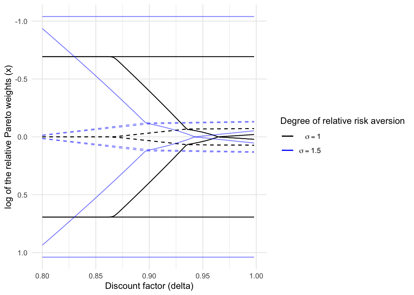

The figure shows that the end-points of intervals shift to left as the degree of relative risk aversion increases.

References

Coate, Stephen, and Martin Ravallion. 1993. “Reciprocity without commitment: Characterization and performance of informal insurance arrangements.” Journal of Development Economics 40 (1): 1–24. https://doi.org/10.1016/0304-3878(93)90102-S.

Kocherlakota, N. R. 1996. “Implications of Efficient Risk Sharing without Commitment.” The Review of Economic Studies 63 (4): 595–609. https://doi.org/10.2307/2297795.

Laczó, Sarolta. 2014. “Does Risk Sharing Increase with Risk Aversion and Risk When Commitment Is Limited?” Journal of Economic Dynamics and Control 46: 237–51.

———. 2015. “RISK SHARING WITH LIMITED COMMITMENT AND PREFERENCE HETEROGENEITY: STRUCTURAL ESTIMATION AND TESTING.” Journal of the European Economic Association 13 (2): 265–92. https://doi.org/10.1111/jeea.12115.

Ligon, Ethan, Jonathan P. Thomas, and Tim Worrall. 2002. “Informal Insurance Arrangements with Limited Commitment: Theory and Evidence from Village Economies.” Review of Economic Studies 69 (1): 209–44. https://doi.org/10.1111/1467-937X.00204.

Marcet, Albert, and Ramon Marimon. 2019. “Recursive Contracts.” Econometrica 87 (5): 1589–1631.