Replication of Thomas & Worrall (1988), Figure 1

Case 1: No overlap

First, I consider the case where there is no overlap ($\omega_{1, upper} < \omega_{2, lower}$). To calculate the end-points of the intervals, evaluate profits at the top of the state 1 interval (where the discounted utility is 0) and utility at the bottom of the state 2 intervals (where the discounted profit is 0). Note that once these end-points are realized, in the next period the contract pays wages $\omega_{1, upper}$ and $\omega_{2, lower}$ with probabilities $p(1)$ and $p(2)$, respectively, and this pattern continues forever. (In some sense this is a steady ``state’’ where contract payments bounce around between $\omega_{1, upper}$ and $\omega_{2, lower}$, but not otehr payments.) The conditions are

$\begin{aligned} &\quad w(1) - \omega_{1,upper} + \frac{\alpha}{1 - \alpha} (p(1) (w(1) - \omega_{1, upper}) + p(2) (w(2) - \omega_{2, lower})) &= 0 \\ &\Leftrightarrow (1 - \alpha) (w(1) - \omega_{1,upper}) + \alpha ((1 - p(2)) (w(1) - \omega_{1, upper}) + p(2) (w(2) - \omega_{2, lower})) &= 0 \\ &\Leftrightarrow (1 - \alpha p(2)) (w(1) - \omega_{1,upper}) - \alpha p(2) (\omega_{2, lower} - w(2))) &= 0 \\ \end{aligned}$

and

$\begin{aligned} &\quad u(\omega_{2,lower}) - u(w(2)) + \frac{\alpha}{1 - \alpha} (p(1) (u(\omega_{1, upper}) - u(w(1))) + p(2) (u(\omega_{2, lower}) - u(w(2)))) &= 0 \\ &\Leftrightarrow (1 - \alpha) (u(\omega_{2,lower}) - u(w(2))) + \alpha (p(1) (u(\omega_{1, upper}) - u(w(1))) + (1 - p(1)) (u(\omega_{2, lower}) - u(w(2)))) &= 0 \\ &\Leftrightarrow \alpha p(1) (u(\omega_{1, upper}) - u(w(1))) - (1 - \alpha p(1)) (u(w(2)) - u(\omega_{2, lower})) &= 0 \end{aligned}$

Below, I define a function to solve this system of equations:

# Define utility function
u <- function(x){
  object <- sqrt(x)
  return(object)
}

# Set the parameter values
w_1 <- 1
w_2 <- 4
p_1 <- 1 / 2
p_2 <- 1 / 2

# For the case where there is no overlap, solve \omega_{2, lower} and \omega_{1, upper}

no_overlap <- function(x, alpha, w_1, w_2, p_1, p_2){
  y <- numeric(2)
  y[1] <- (1 - alpha * p_2)  * (w_1 - x[1]) - alpha * p_2 * (x[2] - w_2)
  y[2] <- alpha * p_1 * (u(x[1]) - u(w_1)) - (1 - alpha * p_1) * (u(w_2) - u(x[2]))
  return(y)
}

Given the function to solve $\omega_{2, lower}$ and $\omega_{1, upper}$, I obtain the value of $\alpha_*$, the cutoff of no-overlap and spot-market-like situations. Also, I calculate the value of $\alpha^*$, the cutoff of no-overlap and overlapping situations.

alpha_vals <- seq(0.50, 0.999, by = 0.0001)
omega_1_upper_vals_no_overlap <- numeric(length(alpha_vals))
omega_2_lower_vals_no_overlap <- numeric(length(alpha_vals))
same_as_spot <- numeric(length(alpha_vals))
x_start <- c((1 + 4) / 2, (1 + 4) / 2)
for (alpha in 1:length(alpha_vals)){
  no_overlap_solutions <- nleqslv(x_start, 
                                  no_overlap, 
                                  alpha = alpha_vals[alpha], 
                                  w_1 = w_1,
                                  w_2 = w_2,
                                  p_1 = p_1,
                                  p_2 = p_2)$x
  omega_1_upper_vals_no_overlap[alpha] <- no_overlap_solutions[1]
  omega_2_lower_vals_no_overlap[alpha] <- no_overlap_solutions[2]
  same_as_spot[alpha] <- is.logical(all.equal(no_overlap_solutions[1], w_1, tolerance = 1e-3))
}

alpha_lower_star <- alpha_vals[max(which(same_as_spot == 1))]
alpha_upper_star <- alpha_vals[min(which(omega_1_upper_vals_no_overlap 
                                         >= omega_2_lower_vals_no_overlap))]

It turned out that $\alpha_*$ is 0.8285, and $\alpha^*$ is 0.9173.

Case 2: Overlapping

Next, I consider the case where there are overlaps. In the same way as above, to calculate the end-points of the intervals, evaluate profits at the top of the state 1 interval (where the discounted utility is 0) and utility at the bottom of the state 2 intervals (where the discounted profit is 0): Note that once these end-points are realized, the future contract payments are unchanged no matter which state realizes (see Proposition 2). The conditions are

$\begin{aligned} &\quad w(1) - \omega_{1,upper} + \frac{\alpha}{1 - \alpha} (p(1) (w(1) - \omega_{1, upper}) + p(2) (w(2) - \omega_{1, upper})) &= 0 \\ &\Leftrightarrow (1 - \alpha) (w(1) - \omega_{1,upper}) + \alpha ((1 - p(2)) (w(1) - \omega_{1, upper}) + p(2) (w(2) - \omega_{1, upper})) &= 0 \\ &\Leftrightarrow \omega_{1,upper} - (1 - \alpha p(2)) w(1) - \alpha p(2) w(2) &= 0 \\ \end{aligned}$

and

$\begin{aligned} &\quad u(\omega_{2,lower}) - u(w(2)) + \frac{\alpha}{1 - \alpha} (p(1) (u(\omega_{2, lower}) - u(w(1))) + p(2) (u(\omega_{2, lower}) - u(w(2)))) &= 0 \\ &\Leftrightarrow (1 - \alpha) (u(\omega_{2,lower}) - u(w(2))) + \alpha (p(1) (u(\omega_{2, lower}) - u(w(2))) + (1 - p(1)) (u(\omega_{2, lower}) - u(w(2)))) &= 0 \\ &\Leftrightarrow u(\omega_{2, lower}) - \alpha p(1) u(w(1)) - (1 - \alpha p(1)) u(w(2)) &= 0 \end{aligned}$

Below I define the function to solve this system of equations:

# For the case where there are overlaps, solve \omega_{2, lower} and \omega_{1, upper}

overlap <- function(x, alpha, w_1, w_2, p_1, p_2){
  y <- numeric(2)
  y[1] <- x[1] - (1 - alpha * p_2) * w_1 - alpha * p_2 * w_2
  y[2] <- u(x[2]) - alpha * p_1 * u(w_1) - (1 - alpha * p_1) * u(w_2)
  return(y)
}

and the end-points at each $\alpha$ are calculated as follows:

alpha_vals <- seq(0.50, 0.999, by = 0.0001)
omega_1_upper_vals_overlap <- numeric(length(alpha_vals))
omega_2_lower_vals_overlap <- numeric(length(alpha_vals))
x_start <- c((1 + 4) / 2, (1 + 4) / 2)
for (alpha in 1:length(alpha_vals)){
  overlap_solutions <- nleqslv(x_start, 
                                  overlap, 
                                  alpha = alpha_vals[alpha], 
                                  w_1 = w_1,
                                  w_2 = w_2,
                                  p_1 = p_1,
                                  p_2 = p_2)$x
  omega_1_upper_vals_overlap[alpha] <- overlap_solutions[1]
  omega_2_lower_vals_overlap[alpha] <- overlap_solutions[2]
}

Replicate the figure

With the information at hand, I replicate Figure 1 in the original paper:

alpha_vals <- seq(0.50, 0.999, by = 0.0001)

omega_1_upper_vals <- numeric(length(alpha_vals))
omega_2_lower_vals <- numeric(length(alpha_vals))
x_start <- c((1 + 4) / 2, (1 + 4) / 2)
for (alpha in 1:length(alpha_vals)){
  # The payments are the same as the spot market wages
  if (alpha_vals[alpha] <= alpha_lower_star){
    omega_1_upper_vals[alpha] <- w_1
    omega_2_lower_vals[alpha] <- w_2
  } else if (alpha_vals[alpha] > alpha_lower_star & alpha_vals[alpha] <= alpha_upper_star){
    omega_1_upper_vals[alpha] <- omega_1_upper_vals_no_overlap[alpha]
    omega_2_lower_vals[alpha] <- omega_2_lower_vals_no_overlap[alpha]
  } else {
    omega_1_upper_vals[alpha] <- omega_1_upper_vals_overlap[alpha]
    omega_2_lower_vals[alpha] <- omega_2_lower_vals_overlap[alpha]
  }
}

omega_1_lower_vals <- rep(w_1, length(alpha_vals))
omega_2_upper_vals <- rep(w_2, length(alpha_vals))

ggplot() +
  geom_line(aes(alpha_vals, omega_1_upper_vals, color="a")) + 
  geom_line(aes(alpha_vals, omega_2_upper_vals, color="b")) + 
  geom_line(aes(alpha_vals, omega_1_lower_vals, color="c")) + 
  geom_line(aes(alpha_vals, omega_2_lower_vals, color="d")) +
  coord_cartesian(xlim = c(alpha_lower_star-0.1, 1.0)) +
  geom_ribbon(aes(x = alpha_vals, ymin = omega_1_lower_vals, ymax = omega_1_upper_vals), 
              fill = "orange", alpha = 0.2) + 
  geom_ribbon(aes(x = alpha_vals, ymin = omega_2_lower_vals, ymax = omega_2_upper_vals), 
              fill = "green", alpha = 0.2) +
  scale_color_manual(name = "End-points", values = c("blue", "purple", "brown", "red"), 
                     labels = c("omega_1_upper", "omega_2_upper", "omega_1_lower", "omega_2_lower")) +
  xlab("Discount factor") +
  ylab("Wages")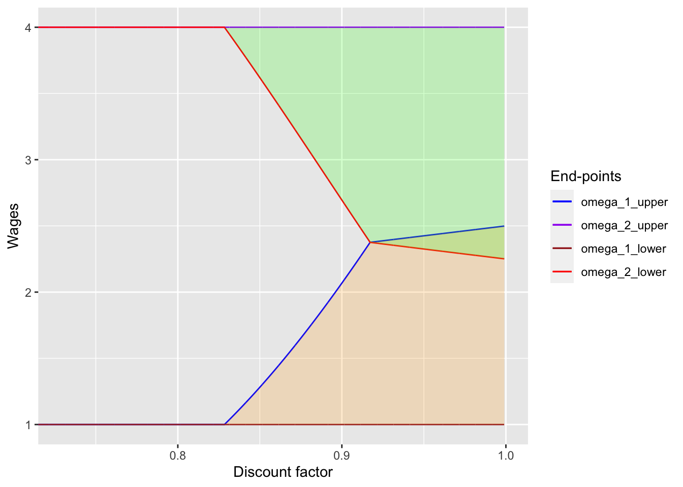

I could replicate the figure! Yay!!

Case 1: No overlap

First, I consider the case where initial wage is high.

w_init <- 3.5
alpha <- 0.9
n <- 5
set.seed(1)
high_wage_dummy <- rbinom(n=n, size=1, prob=0.5)

plot_high_init <- wage_change_plot(w_init, alpha, n, high_wage_dummy)[1]
omega_table_high_init <- wage_change_plot(w_init, alpha, n, high_wage_dummy)[2]
kable(omega_table_high_init, 
      caption = "Realization of spot market wages and the sequence of contract payments")

plot_high_init

## [[1]]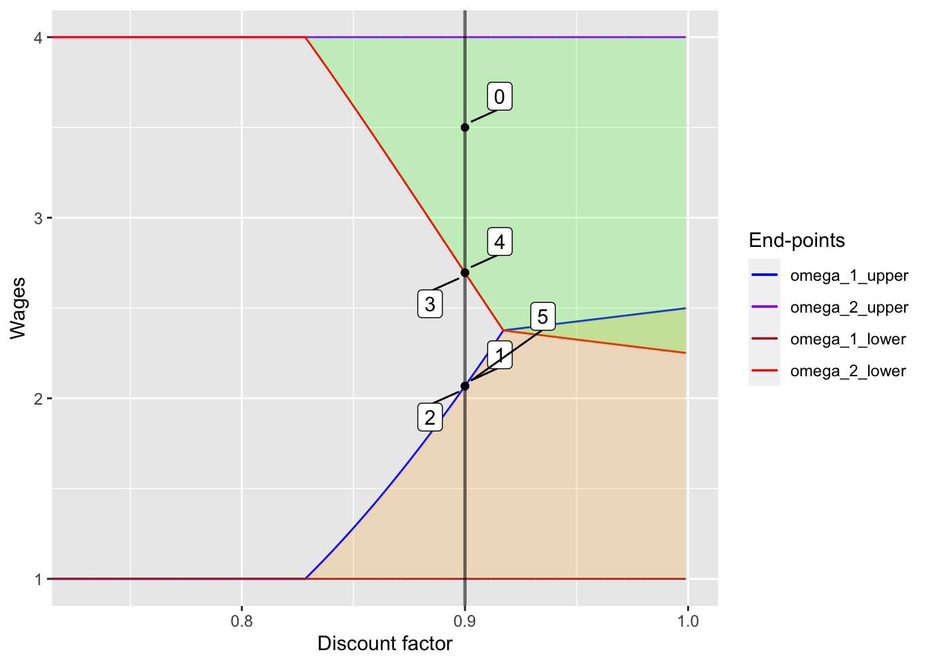

The table shows the change in contract payments and spot market wages. Also, the table shows how contract wages update.

Next, I consider the case where initial wage is between $\omega_{2, lower}$ and $\omega_{1, upper}$.

w_init <- 2.35
alpha <- 0.9
n <- 5
set.seed(2)
high_wage_dummy <- rbinom(n=n, size=1, prob=0.5)

plot_med_init <- wage_change_plot(w_init, alpha, n, high_wage_dummy)[1]
omega_table_med_init <- wage_change_plot(w_init, alpha, n, high_wage_dummy)[2]
kable(omega_table_med_init, 
      caption = "Realization of spot market wages and the sequence of contract payments")

plot_med_init

## [[1]]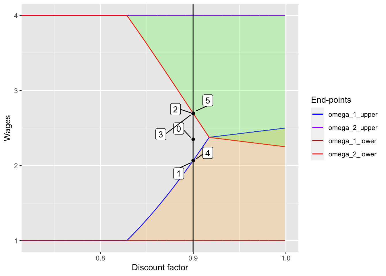

In this case, except for the initial wage, the contract payments bounce back and force between $\omega_{2, lower}$ and $\omega_{1, upper}$, depending on the spot market wage at the period.

Case 2: Spot-market-like wages

Next, I move on and see what would happen if we have a low discount factor.

w_init <- 3.5
alpha <- 0.8
n <- 5
set.seed(1)
high_wage_dummy <- rbinom(n=n, size=1, prob=0.5)

plot_high_init <- wage_change_plot(w_init, alpha, n, high_wage_dummy)[1]
omega_table_high_init <- wage_change_plot(w_init, alpha, n, high_wage_dummy)[2]
kable(omega_table_high_init, 
      caption = "Realization of spot market wages and the sequence of contract payments")

plot_high_init

## [[1]]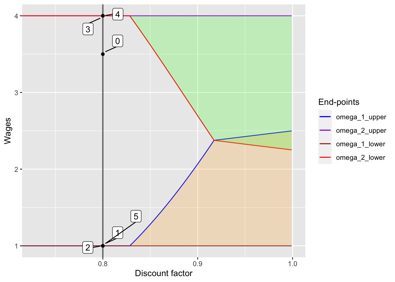

As one can see, the wage completely co-moves with spot markets wages.

Case 3: Overlapping regions

Finally, I will try the high discount factor and see how the wages change in the overlapping region. I will show figures and tables with low and medium initial wages.

w_init <- 1.5
alpha <- 0.95
n <- 5
set.seed(1)
high_wage_dummy <- rbinom(n=n, size=1, prob=0.5)

plot_low_init <- wage_change_plot(w_init, alpha, n, high_wage_dummy)[1]
omega_table_low_init <- wage_change_plot(w_init, alpha, n, high_wage_dummy)[2]
kable(omega_table_low_init, 
      caption = "Realization of spot market wages and the sequence of contract payments")

plot_low_init

## [[1]]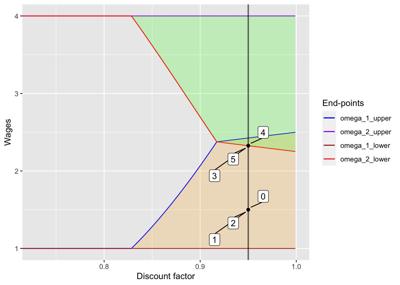

w_init <- 2.35
alpha <- 0.95
n <- 5
set.seed(1)
high_wage_dummy <- rbinom(n=n, size=1, prob=0.5)

plot_med_init <- wage_change_plot(w_init, alpha, n, high_wage_dummy)[1]
omega_table_med_init <- wage_change_plot(w_init, alpha, n, high_wage_dummy)[2]
kable(omega_table_med_init, 
      caption = "Realization of spot market wages and the sequence of contract payments")

plot_med_init

## [[1]]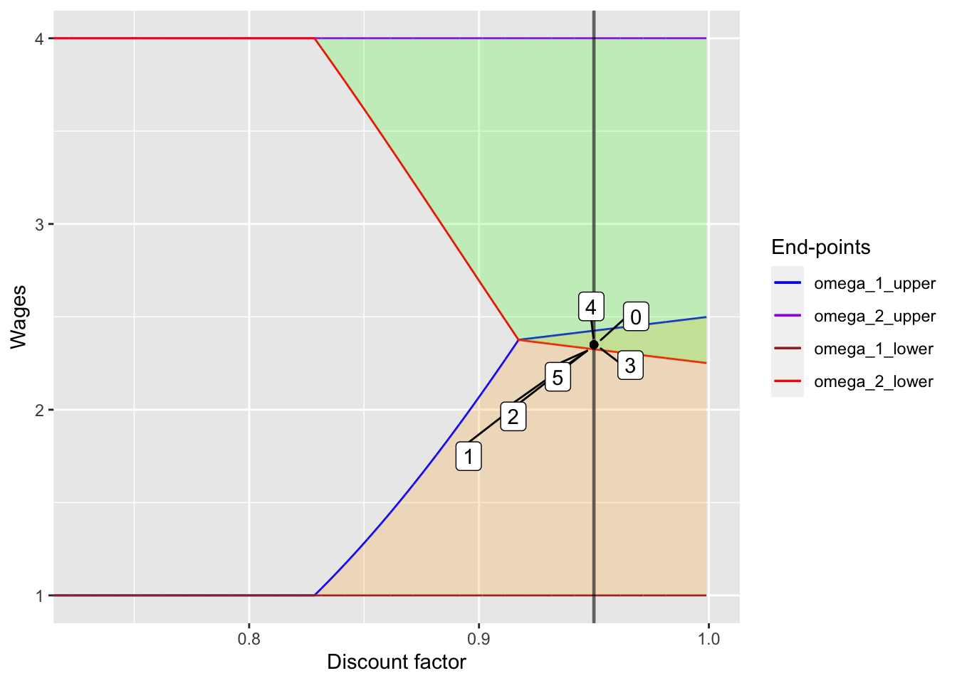

In the first figure, once the wage lies between $\omega_{2, lower}$ and $\omega_{1, upper}$, the wages stays there forever no matter what the spot market wages are. It should be noted that this corresponds to back-loading wage schemes, where wages increase from low to high over time. In the second figure, since the initial wage already lies between $\omega_{2, lower}$ and $\omega_{1, upper}$, the wages stays at the initial point.