pacman::p_load(
  tidyverse,
  pracma,
  latex2exp,
  ggrepel
)3 Risk sharing with limited commitment and storage: Simulation
Based on the numerical solution from the previous section, I simulate an income stream to see how storage and consumption change over time.
3.1 Code
3.1.1 Global settings
4 Load solution
modelSolutionList <- readRDS(
  file.path('IntermediateData/modelSolution.rds')
)
relativeParetoWeightsBoundsArray <- modelSolutionList[[3]]
nextStorageArray <- modelSolutionList[[4]]
incomeSeq <- sample(seq(1, numStates), size = simSize, replace = TRUE)
storageSeq <- c(0)
relativeParetoWeightSeq <- c(1)
consHH1Seq <- c()
for (i in seq(1, simSize)) {
storageSeq <- c(
storageSeq,
interp2(
x = storageGridPoints,
y = relativeParetoWeightsGridPoints,
Z = nextStorageArray[incomeSeq[i], , ],
xp = storageSeq[i] %>%
pmin(max(storageGridPoints)) %>%
pmax(min(storageGridPoints)),
yp = relativeParetoWeightSeq[i] %>%
pmin(max(relativeParetoWeightsGridPoints)) %>%
pmax(min(relativeParetoWeightsGridPoints)),
method = "linear"
)
)
relativeParetoWeightSeq <- c(
relativeParetoWeightSeq,
relativeParetoWeightSeq[i] %>%
pmax(
approx(
storageGridPoints,
relativeParetoWeightsBoundsArray[
1,
incomeSeq[i],
],
storageSeq[i],
rule = 2
)$y
) %>%
pmin(
approx(
storageGridPoints,
relativeParetoWeightsBoundsArray[
2,
incomeSeq[i],
],
storageSeq[i],
rule = 2
)$y
)
)
consHH1Seq <- c(
consHH1Seq,
calculateHH1Consumption(
(
aggregateIncomeGridPoints[incomeSeq[i]]
+ (1 + returnOnStorage) * storageSeq[i]
- storageSeq[i + 1]
),
relativeParetoWeightSeq[i + 1],
sigma
)
)
}
simulationResult <- tibble(
period = seq(1, simSize),
income = incomeSeq,
storage = storageSeq[2:(simSize + 1)],
consHH1 = consHH1Seq
) %>%
mutate(
previousIncome = lag(income),
changeIncome = paste(as.character(previousIncome), '->', as.character(income))
)4.1 Storage and consumption at the steady state
First I show the storage and consumption at the steady state. The figures below show that, even in the steady state, they are stochastic. This is in contrast to the implication of a limited commitment model without storage, as in Kocherlakota (1996), where consumption in limit takes a finite number of values. Also, the stochastic consumption clearly shows the violation of the “amnesia” property in Kocherlakota (1996): consumption is not determined by the state and identities of households whose participation constraints are binding.
simulationResult %>%
  filter(period >= 100) %>%
  ggplot(aes(x = period, y = storage)) +
  geom_point() +
  xlab('Time period') +
  ylab('Public storage') +
  theme_classic()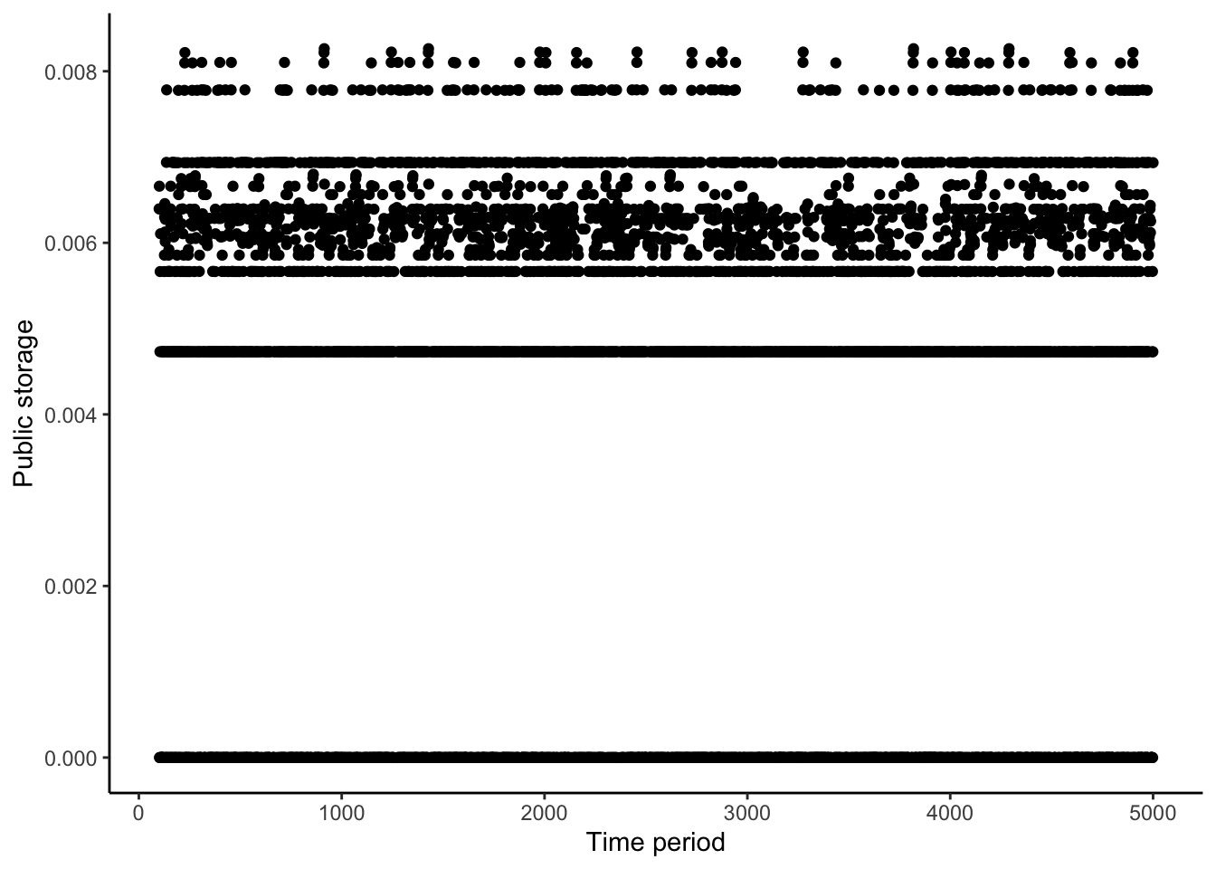
simulationResult %>%
  filter(period >= 100) %>%
  ggplot(aes(x = period, y = consHH1)) +
  geom_point() +
  xlab('Time period') +
  ylab('HH1 consumption') +
  theme_classic()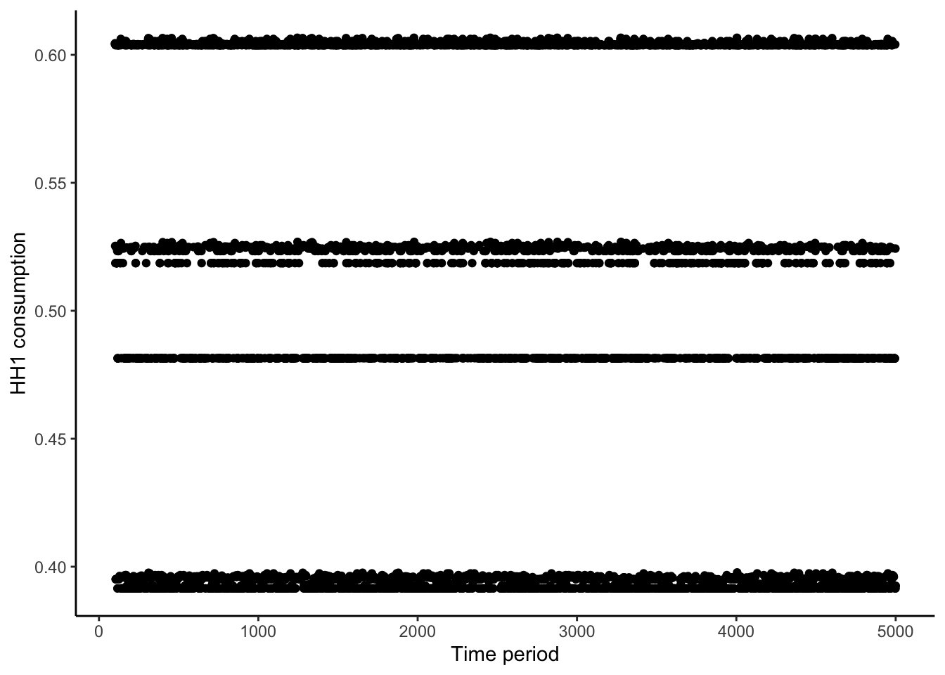
4.2 Relative Pareto weight intervals
The figure below shows the interval bounds of relative Pareto weights, where the x-axis is public storage. It shows that when public storage is large, participation constraints are more relaxed and hence more transfers are achievable. This is exactly why the social planner has an incentive for saving: more public storage allows a better functionality of a risk-sharing network.
tibble(
  storage = storageGridPoints,
  x_l_1 = relativeParetoWeightsBoundsArray[1,1,],
  x_l_2 = relativeParetoWeightsBoundsArray[1,2,],
  x_l_3 = relativeParetoWeightsBoundsArray[1,3,],
  x_h_1 = relativeParetoWeightsBoundsArray[2,1,],
  x_h_2 = relativeParetoWeightsBoundsArray[2,2,],
  x_h_3 = relativeParetoWeightsBoundsArray[2,3,]
) %>%
  ggplot() +
  geom_line(aes(x = storage, y = x_l_1, color = 'a')) +
  geom_line(aes(x = storage, y = x_l_2, color = 'b')) +
  geom_line(aes(x = storage, y = x_l_3, color = 'c')) +
  geom_line(aes(x = storage, y = x_h_1, color = 'd')) +
  geom_line(aes(x = storage, y = x_h_2, color = 'e')) +
  geom_line(aes(x = storage, y = x_h_3, color = 'f')) +
  scale_color_manual(
      name = "End-points",
      values = c(
        "blue",
        "purple",
        "brown",
        "red",
        "orange",
        "gray"
        ),
      labels = unname(TeX(c(
        "$\\underline{x}_1$",
        "$\\underline{x}_2$",
        "$\\underline{x}_3$",
        "$\\bar{x}_1$",
        "$\\bar{x}_2$",
        "$\\bar{x}_3$"
        )))
      ) +
  theme_minimal() +
  scale_y_log10() +
  xlab('Public storage') +
  ylab('Relative Pareto weight')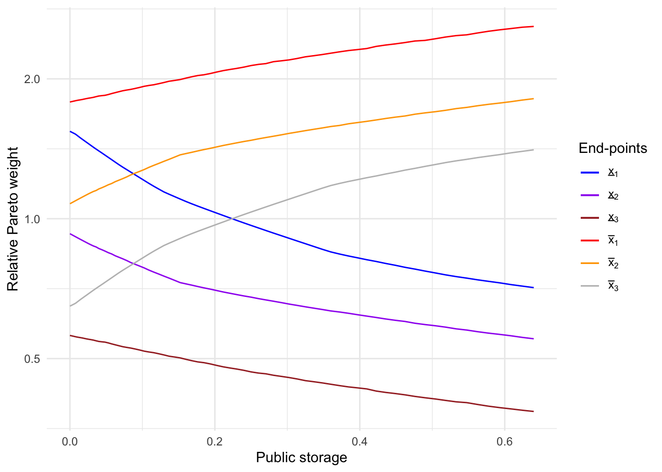
4.3 Storage behavior
This is not a simulation result, but let me know how the storage policy function looks differently by income states. The first is for the case where the relative Pareto weight is 1.
tibble(
  storage = storageGridPoints,
  x1 = nextStorageArray[1,101,],
  x2 = nextStorageArray[2,101,],
  x3 = nextStorageArray[3,101,],
) %>%
  filter(storageGridPoints < 0.05) %>%
  ggplot() +
  geom_line(aes(x = storage, y = x1, color = 'a')) +
  geom_line(aes(x = storage, y = x2, color = 'b')) +
  geom_line(aes(x = storage, y = x3, color = 'c')) +
  xlab("Current public storage") +
  ylab("Next-period public storage") +
  scale_color_manual(
      name = "Income states",
      values = c(
        "blue",
        "red",
        "orange"
        ),
      labels = c(
        "Low HH1 income",
        "Medium HH1 income",
        "High HH1 income"
      )
      ) +
  theme_minimal()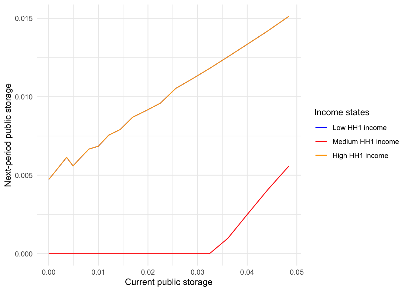
And this is the case where the relative Pareto weight is 0.64. Remember that a smaller relative Pareto weight is in favor of Household 1.
tibble(
  storage = storageGridPoints,
  x1 = nextStorageArray[1,51,],
  x2 = nextStorageArray[2,51,],
  x3 = nextStorageArray[3,51,],
) %>%
  filter(storageGridPoints < 0.05) %>%
  ggplot() +
  geom_line(aes(x = storage, y = x1, color = 'a')) +
  geom_line(aes(x = storage, y = x2, color = 'b')) +
  geom_line(aes(x = storage, y = x3, color = 'c')) +
  xlab("Current public storage") +
  ylab("Next-period public storage") +
  scale_color_manual(
      name = "Income states",
      values = c(
        "blue",
        "red",
        "orange"
        ),
      labels = c(
        "Low HH1 income",
        "Medium HH1 income",
        "High HH1 income"
      )
      ) +
  theme_minimal()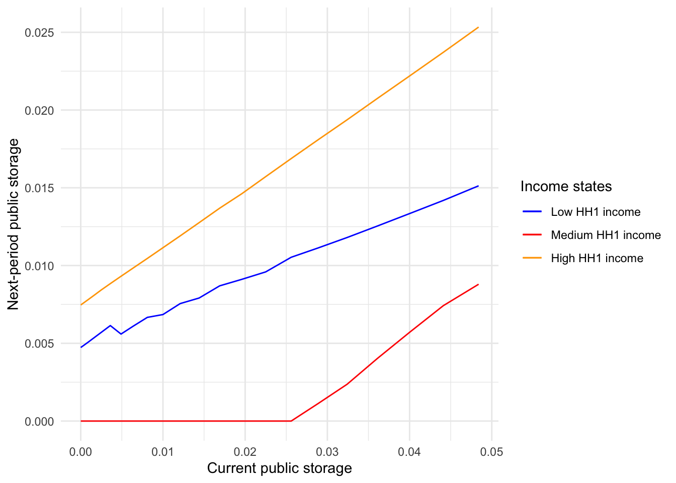
4.4 Transition in storage
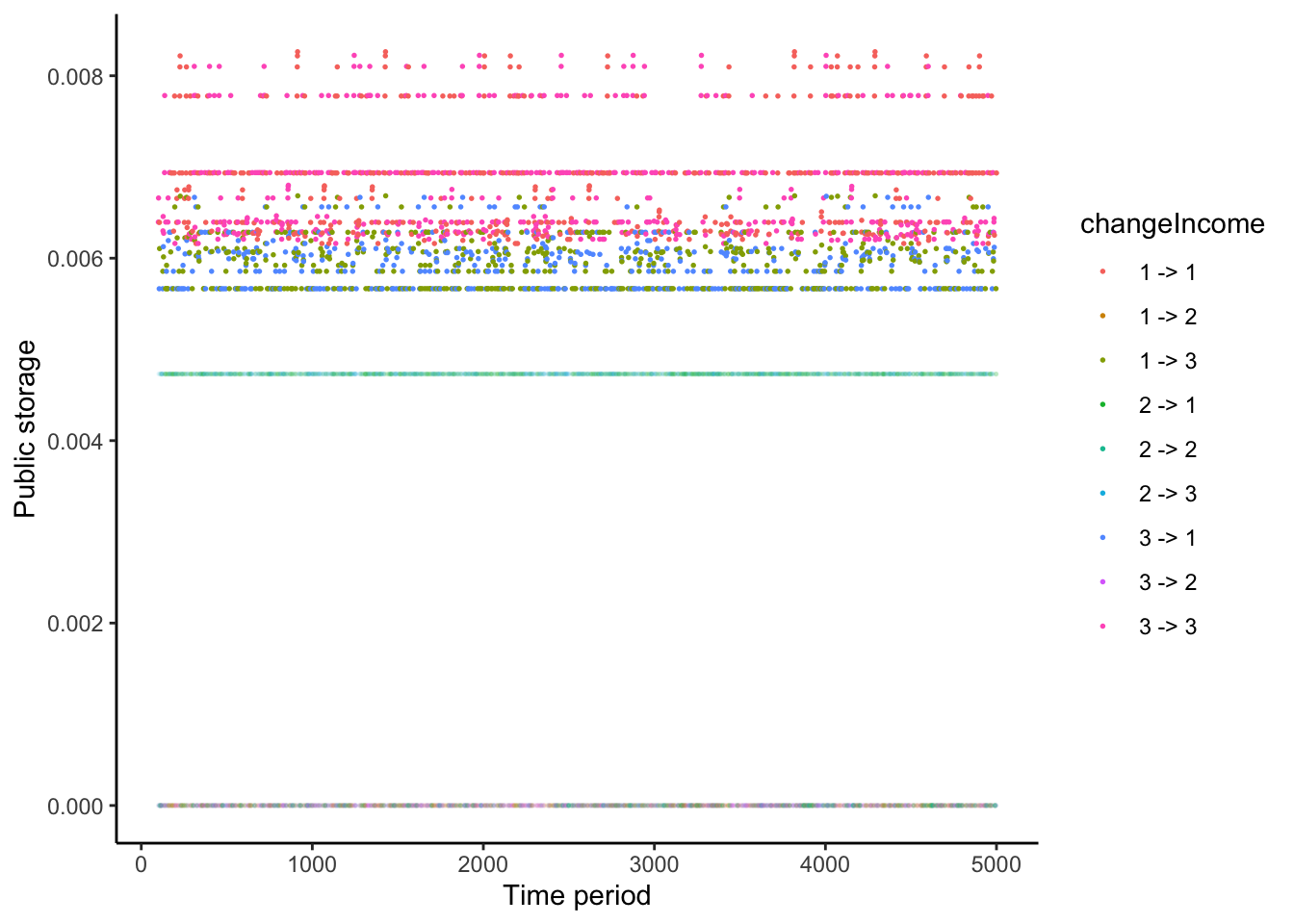
Here, I show how storage evolves over time, depending on the sequence of income realizations. The figure uses different colors for different sequences (state 1: low HH1 income, state 2: medium HH1 income, state 3: high HH1 income).
simulationResult %>%
  filter(period >= 100) %>%
  mutate(cond = (income == 2)) %>%
  ggplot() +
  geom_point(aes(x = period, y = storage, color = changeIncome), size = 1.0) +
  xlab('Time period') +
  ylab('Public storage') +
  theme_classic()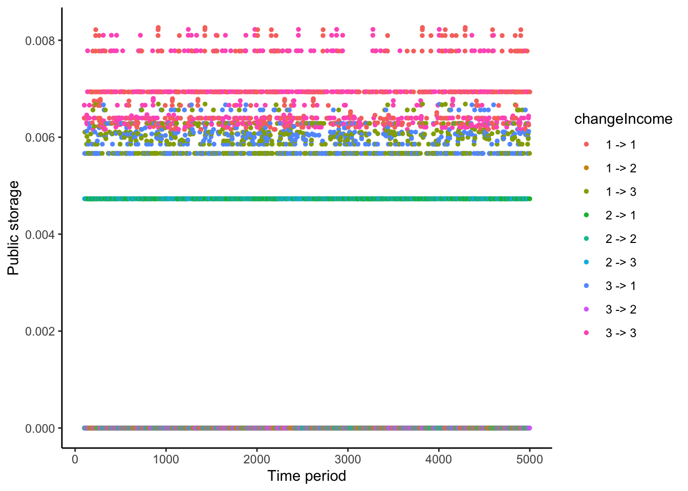
4.4.1 No income inequality state
When the income state 2 is realized, income is equal between two households, and the social planner stores nothing for the following period.
simulationResult %>%
  filter(period >= 100) %>%
  mutate(cond = (income == 2)) %>%
  mutate(alpha = 1 * cond + 0.01 * (!cond)) %>%
  ggplot() +
  geom_point(aes(x = period, y = storage, color = changeIncome, alpha = alpha), size = 0.3) +
  scale_alpha(guide = "none") +
  xlab('Time period') +
  ylab('Public storage') +
  theme_classic()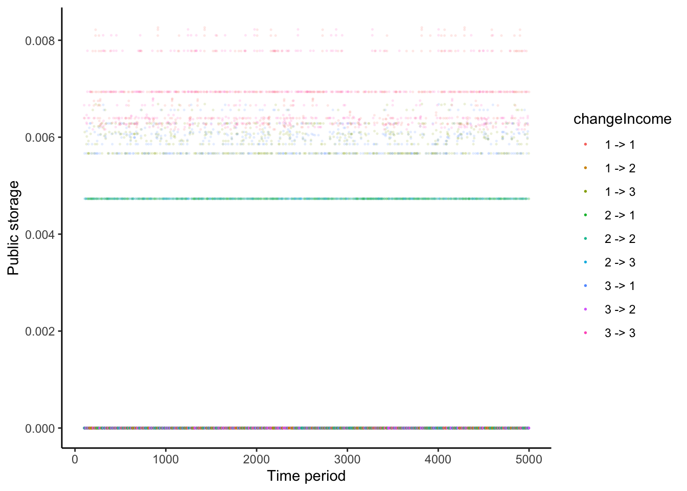
4.4.2 From no income inequality to some inequality
When a medium income state is followed by an income state with inequality, the social planner makes savings.
simulationResult %>%
  filter(period >= 100) %>%
  mutate(cond = (income != 2 & previousIncome == 2)) %>%
  mutate(alpha = 1 * cond + 0.2 * (!cond)) %>%
  ggplot() +
  geom_point(aes(x = period, y = storage, color = changeIncome, alpha = alpha), size = 0.3) +
  scale_alpha(guide = "none") +
  xlab('Time period') +
  ylab('Public storage') +
  theme_classic()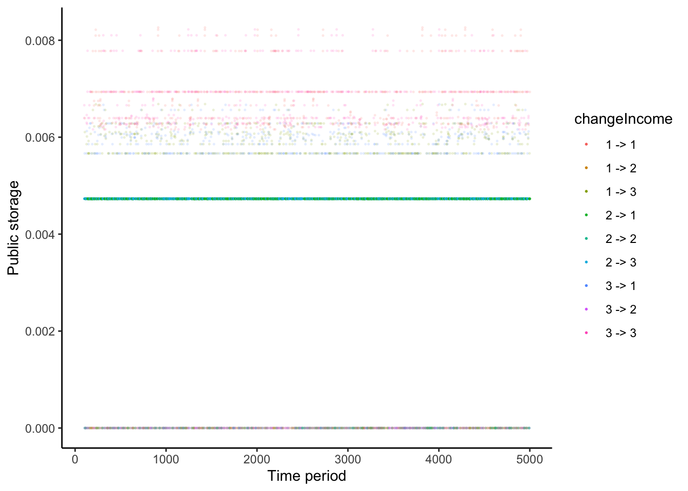
4.4.3 Consecutvive states with some income inequality
When unequal income states continue, more assets are accumulated.
simulationResult %>%
  filter(period >= 100) %>%
  mutate(cond = (income != 2 & previousIncome != 2)) %>%
  mutate(alpha = 1 * cond + 0.2 * (!cond)) %>%
  ggplot() +
  geom_point(aes(x = period, y = storage, color = changeIncome, alpha = alpha), size = 0.3) +
  scale_alpha(guide = "none") +
  xlab('Time period') +
  ylab('Public storage') +
  theme_classic()